


How To Use VLOOKUP In Excel: Here Is The Easy Way
The vlookup is the best function of excel and in the present time, most of the people use the vlookup. but most people have heard about the option function but no one knows about what it does and where it is used. A built-in Excel function that is designed to organize columns together.
The values in one column of information, and returns the comparing value from another Column. All the more, in fact, the VLOOKUP work looks into a value in the start Column of a given range and returns a value in a similar line from another Column. Simply put, the Vlookup is a database function for excel it uses to find the column and row in a table. how it works to break down for remember.
How to use Vlookup in Microsoft Excel
- Identify a Column of cells you’d prefer to load up with new information.
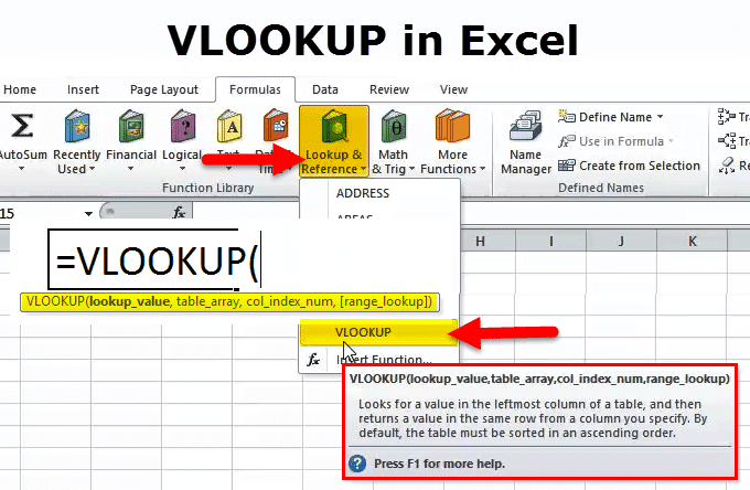
- Select ‘function’ (Fx) > VLOOKUP and addition this equation into your featured cell.
- You have to enter the query a value for which you need to recover new information.
- Enter the table array of the spreadsheet where your ideal information the Address.
- Enter the column number of the information you need Excel to return.
- First of all, enter your range query to locate a correct or approximate match of your query Value.
- Click on Enter Button.
- After that fill your new Column in Excel.
Identify a column of cells you’d like to fill with new information
| Custome name | Email Address | Date signed | MRR |
| Brian | Brain@gmail.com | 26/4/2018 | |
| Chris | Chris@gmail.com | 12/5/2018 | |
| Chris Carozza | Chris12@gmail.com | 24/6/2018 | |
| Benjamin Fisher | Benjamin@gmail.com | 16/4/2018 | |
| Karen | karen@gmail.com | 26/4/2018 | |
| Hugo | Hugo@gmail.com | 26/8/2018 | |
| Aaron | Arron@gmail.com | 6/9/2018 |
In this information is originating from a rotate table made in Excel, duplicate the information into a new spreadsheet so the VLOOKUP function can uninhibitedly peruse this information.
Then, label a column next to the cells you need more data on with an appropriate title in the top cell, for example, “MRR,” for a month to month repeating income. This new section is the place the information you’re bringing will go.
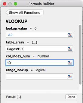
Enter the query a value for which you need to recover new information.
The main criteria are your query value – this is the estimation of your spreadsheet that has information related to it, which you need Excel to discover and return for you. To enter it, click on the cell that conveys a worth you’re attempting to discover a counterpart for. In our model, it appeared over, it’s in cell A2. You’ll begin relocating your new information into D2 since this cell speaks to the MRR of the client name recorded in A2.
Enter the table array of the spreadsheet where your desired information is located.
the “table exhibit” field, enter the scope of cells you’d prefer to look and the sheet where these cells are found, utilizing the organization appeared in the screen capture above. The passage above methods the information we’re searching for is in a spreadsheet titled “Pages” and can be found anyplace between segment B and segment K.
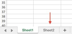
The sheet where your information is found must be inside your current Excel document.
This implies your information can either be in an alternate table of cells someplace in your present spreadsheet, or in an alternate spreadsheet connected at the base of your exercise manual, as demonstrated as follows.
For example, if your information is an address in “Sheet 2” between cells C6 or L20, your table array entry will be “Sheet2!C6: L20.”
Enter the column number of the information you want Excel to return.
Underneath the table array field, you’ll enter the “column file number” of the table array you’re looking through. For Example, in case you’re concentrating on column B through K (recorded “B: K” when entered in the “table array” field), yet the particular qualities you need are in column K, you’ll enter “10” in the “Column file number” field since segment K is the tenth column from the left.
VLOOKUP syntax
VLOOKUP(lookup_value, table_array, col_index_num, [range_lookup])
Value - The value to search for in the start column of a table.
Table - The table from which to recover value.
col_index - The column in the table from which to recover value.
Range_lookup - [optional] TRUE = inexact match (default). FALSE = accurate match.
- V=Virtical
- LOOKUP = is to look up a value.
For example is a rundown of three columns, Name, Address, Telephone Number, where your value to discover is “Name” and the value to return is “Phone Number.” You are looking to just return harry phone number, and not his location. The capacity would resemble this: As you see, the capacity has 4 components – the initial three are required and the last one is discretionary.
=VLOOKUP(“harry”,A1:C20,3,True)
VLOOKUP will work in three steps
- find the “name” Column, Column 1 For ” harry ” And stops at that row
- When finding the name, the Vlookup function scan across the same row find in 1 and jumps to 4th column (mobile number)
- The vlookup function returns the value it found in(2)
A vlookup function is a lovely tool for a very organized database in a very simple table. When you want to use any disorganized data or have several repeated values, or on the other hand need to look to one side or to one side of the datapoint you scan for, progressively mind-boggling (and incredible!) capacities should be utilized, similar to Index-Match.
A VLOOKUP function exists of four components
- The range where you need to discover the worth and the arrival esteem;
- The worth you need to gaze upward;
- The quantity of the column inside your defined range, that contains the arrival value;
- 0 or FALSE for a definite match with the worth you are searching for; 1 or TRUE for an inexact match.
The Formula Always Searches to the right
When Conducting a VLOOKUP in Excel, you’re basically searching for new information in an alternate spreadsheet that is related to old information in your ebb and flow one. When VLOOKUP runs this inquiry, it generally searches for the new information to one side of your momentum information.
For example, if one spreadsheet has a vertical rundown of names, and another spreadsheet has a sloppy list of those names and their email addresses, you can utilize VLOOKUP to recover those email addresses in the request you have them in your first spreadsheet. Those messages tend to must be recorded in the segment to one side of the names in the subsequent spreadsheet, or Excel won’t have the option to discover them.
Conclusion
Given information is beneficial and helpful for you. Vlookup is the best function of excel. The function we use in the Microsoft Excel function. This function is used in most of the company because there is no problem in adding the salary of the worker to it and as per his presentation, it should be accounted for.
A built-in Excel function that is designed to organize columns together. The values in one column of information, and returns the comparing value from another Column. and that simply put, the Vlookup is a database function for excel it uses to find the column and row in a table. how it works to break down for remember.